This blog post has been written by Dr. Jing Zhang, adopted from research she presented with Dr. Thomas Fisher and Qi He, Miami University masters student.

Linear regression is likely to be the first statistical modeling tool that many of you learn in your coursework, no matter you are a data science and statistics major, math and stat major, analytics co-major or data analytics major. It is still a popular modeling tool because it is easy to implement mathematically/computationally, and the model findings are intuitive to interpret. However, it also suffers from the lack of flexibility due to all the important model assumptions that are possibly problematic in real analysis: normality of responses, independence among observations, linear relation between the response and group of predictors. When outliers exists in the data, or the predictors are highly correlated with each other, the model findings will be distorted and therefore misleading in decision-making. What’s more, it suffers more in the “big-data” era.

A real “BIG” data set would be too big to hold in a single computer’s memory, while a “big” data simply mean that the data set is so big that the traditional statistical analysis tools, such as the linear regression model, would be too time consuming to implement, and suffers more from the rounding errors in computation.

Big data sets often have many variables, i.e. a lot of predictors in the linear regression model (i.e., large “p”), in addition to the large number of data observations (i.e., large “n”). Therefore, we need to select the “true” signals among lots “noises” when fitting any statistical models to such a data set, in another word, we often need to conduct “variable selection.” We wish to speed up the model fitting, variable selection and prediction in analysis of big data sets, yet with relatively simple modeling tools, such as linear regression.

Popular choices involves subsampling the big data and focusing on the analysis of the subset of information. For example, bags of little bootstraps (Kleiner et al. 2014) suggested selecting a random sample of the data and then using bootstrap on the selected sample to recover the original size of the data in the following analysis, which would effectively reduce the memory required in the data storage and analysis, and help in the “BIG” data case.

In addition to random selection, researchers also suggested using sampling weights based on the features of data observation, such as the leverage values (Ma and Sun, 2014) to retain the feature of the data set as much as we can when the subsampling has to be done.

Alternatively, the “divide and conquer” idea has also been popular:  big data are split into multiple blocks of smaller sample size without overlap and the analysis results of each block are then aggregated to obtain the final estimated model and predictions (Chen and Xie, 2014). This idea utilizes all the information in the data sets. In a CADS funded project, we explore the revamping of linear regression in big data predictive modeling using a similar “divide and resample” idea, via a two-stage algorithm. Firstly, we combine the least absolute shrinkage and selection operator (LASSO) (Tibshirani, 1996), which helps select the relevant features; and the divide and conquer approach, which helps deal with the large sample size, in the variable selection stage, with products being the selected relevant features in the big data with high dimension. Secondly, in the prediction stage, with the selected features, when the data are of extremely high sample size, we subsample the data multiple times, refit the model with selected features to each subsample, and then aggregate the predictions based on the analysis of each subsample. When the data are sizable but the chosen model can still be fitted with reasonable computing cost, predictions are obtained directly by refitting the model with selected features to the complete data. Here is the detailed description of the algorithm:

Step 1. Partition a large data set of sample size  into  blocks, each with sample size . The samples are randomly assigned to these blocks.

Step 2. Conduct variable selection with LASSO in each block individually.

Step 3. Use “majority voting” to select the variables, i.e, if we have a “majority” of blocks end up selecting a predictor variable in the analysis, this predictor is retained.

Step 4. When “” is large but still can be handled as one piece, refit the model with selected variables to the original data and predict based on the parameter estimates. When “” is too large to be handled as one piece, randomly select multiple subsample from the original data and refit the model with selected variables on the subsamples, then aggregate the predictions based on the models fitted to different subsamples (e.g. mean or median of the predicted values).

Simulation studies are often used to evaluate the performance of statistical models, methods and algorithms. In a simulation study, we are able to simulate “plausible” data from a known probabilistic framework with pre-picked values of model parameters. Then the proposed statistical analysis method would be implemented to fit the simulated data, and the analysis findings, such as the estimated parameters, predicted responses of a holdout set, would be compared with the true values we know in the simulation. When many such plausible data sets are simulated and analyzed, we are able to empirically evaluate the performance of the proposed methods through the discrepancy between the model findings and true values. In this project, we conducted a simulation study to help make important decisions on key components of the proposed algorithm, including the number of blocks we divide the complete data into, and how to decide “majority” in the variable selection step. This simulation study was also designed such that we are able to evaluate the impact of multicolinearity (highly correlated predictors) and effect size (strength of the linear relation between response and predictors) on the performance of the proposed algorithm in variable selection and prediction.

We simulated responses from 11,000 independent data observations total from a normal population, with a common variance of 2, among which 10,000 observations are chosen as the training set and the remaining 1,000 observations are used as the test set. For each of the 11,000 data observations, a vector of 500 predictors are simulated from normal population with mean 0, and a covariance matrix, . Two different setup of  were used, with the first one being a diagonal identity matrix, indicating a “perfect” scenario with complete independence among the predictors; and a second one being a matrix whose entry in row  and column  is determined by , mimicking a “practical” scenario where the nearby predictors are highly correlated (AR(0.9) correlation structure). Among the 500 predictors, 100 are randomly chosen to be the “true” signals and three different sets of true regression coefficients (i.e. the effect size) are chosen as follows to evaluate the ability of our proposed two-stage algorithm in terms of capturing the “true” signals when the signals are stronger (i.e., larger effect size) vs. weaker (i.e., smaller effect size). The remaining 400 predictors are all associated with zero regression coefficients in the “true” model that generates the data.

1. all 100 regression coefficients are equal to 2;
2. all 100 regression coefficients are equal to 0.75;
3. 50% of regression coefficients are randomly chosen to be 0.75 and the rest are set to be 2.

 Let’s summarize what we wish to do with this simulation study:

• How many block should we divide the 10,000 training set observations into? (4 blocks of 2,500 observation each? 5 blocks? 8,10, 16, 20 or 25 blocks?)

• What is a good threshold for “majority voting?” Analyses of % of the blocks suggest selecting a variable. %= 50%? 60%? …100%?)
• How does the effect size impact the variable selection and prediction?
• How does multicolinearity impact the variable selection and prediction?

To compare the performance of the proposed method under different setups, we evaluated the following quantities: 

• Sensitivity (proportion of the “true signals” picked up by the method, i.e. how many out of the 100 predictors impacting the mean of response are selected) and specificity (proportions of the 400 “non-signal” predictors not selected by the method) of variable selection
• Mean squared predictor error (MSPE) of the test set.

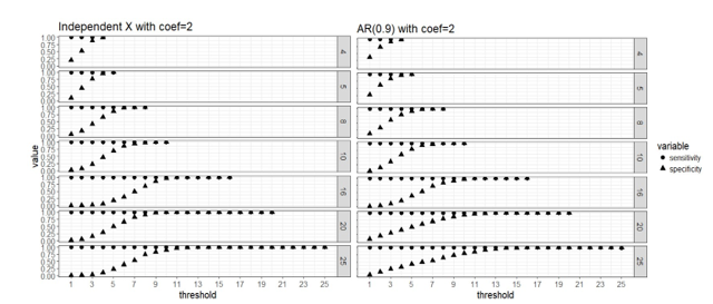
Here are four graphs that help us visualize the simulation study findings on the determination of “majority” when different number of blocks are used. 

Figure 1. Strong signal scenario (regression coefficients are all equal to 2): sensitivity and specificity of the two-stage algorithm when training set are divided into  blocks respectively, and a variable is selected when  out of  blocks selects this predictor, where  =4, 5, 8, 10, 16, 20 and 25, = . Both the case with complete independence among predictors (left panel) and correlated predictors (right panel) are presented.

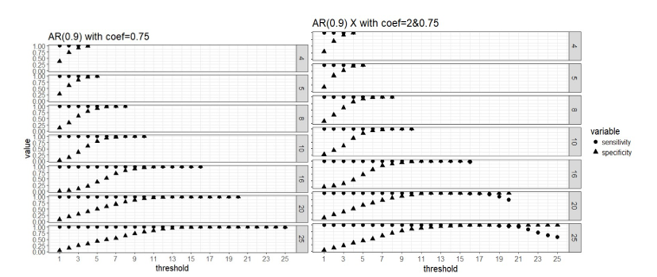
Figure 2. Weak signal scenario (regression coefficients are all equal to 0.75, left panel) and mixed signal scenario (regression coefficients are 0.75 or 2, right panel) with correlated predictors: sensitivity and specificity of the two-stage algorithm when training set are divided into  blocks respectively, and a variable is selected when  out of  blocks selects this predictor, where  =4, 5, 8, 10, 16, 20 and 25, = .

Apparently that when parallel computing is possible, it is computationally cheaper to divide the data into more blocks as there are less observations in each block and the computation speed is restricted by the computing cost of fitting the model to each block. Our simulation study did not use a real “BIG” sample size, so the computing time for each block is not high even when we use as low as 4 block. But in practice it is possible that we have giant training data and need to lower the computing cost of fitting a linear regression to a single block because the blocks still have large samples. All the number of blocks we considered here seem to approach the same level of sensitivity and specificity in variable selection, and it seems that 50% or higher blocks agreeing on the selection of variables is a good threshold for “majority voting.”

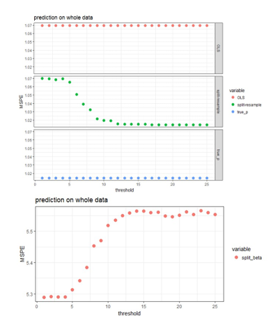
Four approaches are compared for the case of using 25 blocks on the data with independent predictors when the effect sizes are 2 (strong signal scenario).  

1. OLS: fit OLS with all 500 predictors to the original  
2. Split-resample: fit OLS with selected variables in the proposed approach to the original data
3. True p: fit OLS with the 100 “true signals” to the original data 
4. Split-resample: predict with aggregated estimation function in Chen and Xie (2014)

Comparison of the prediction performance can be visualized in the following figures:

Figure 3: MSPE computed by refitting the model with selected variables to the original data and predict for the hold out test set.

The aggregated predictions result in much higher MSPE compared to the other three approaches, so it is shown in the lower panel of Figure 3, while the other three approaches are shown in the upper panel of Figure 3. The proposed approaches produces MSPE that approaches the best scenario when we know exactly which subset of the predictors are “true signals” in the simulated data when majority voting is used assuming 50% or higher proportion of blocks is the threshold of selecting predictors. It seems that the proposed algorithm works well in variable selection when the predictors are independent or correlated; and also predicts well when 50% or higher proportion of blocks is the threshold of selecting predictors. The smaller the effect size, the more blocks need to agree on variable selection in order to achieve the same sensitivity and specificity, but this 50% or higher threshold seem to work for both strong and weak signal case in general.

About the Author

This blog post is reproduced from ISI Statisticians React to the News blog (https://blog.isi-web.org/react). It was released on 25 August 2020

Michael DeWine, governor of the state of Ohio in the United States, provided a visible example of the  properties of screening tests.

Gov. Mike DeWine of Ohio Tests Positive, Then Negative, for Coronavirus by Sarah Mervosh, The New York Times (6 August 2020 with 7 August 2020 update).

After testing positive for COVID-19 on a rapid antigen test, he missed an opportunity to meet with the US president who was visiting DeWine’s state. After DeWine was tested again using a slower, more accurate (RT-PCR) test, he was negative for COVID-19. A additional test administered a day later also was negative.

Are there benefits in having a rapid, less accurate test as well as having a slower, more accurate test? Let’s consider what accuracy means in these tests and why you might be willing to tolerate different errors at different times. 

I won’t address how these tests are evaluating different biological endpoints. I’ve been impressed at how national and local sources have worked to explain the differences between tests that look for particular protein segments or for genetic material characteristic of the virus. Richard Harris (National Public Radio in the US) also provided a nice discussion of reliability of COVID-19 tests that might be of interest. 

I want to talk about mistakes, errors in testing. No test is perfectly accurate. Accuracy is good but accuracy can be defined in different ways, particularly in ways that reflect errors in decisions that are made. Two simple errors are commonly used when describing screening tests – saying someone has a disease when, in truth, they don’t (sorry Governor DeWine) or saying someone is disease free when, in truth, they have the disease. Governor DeWine had 3 COVID-19 tests – the first rapid test was positive, the second and third tests were negative. Thus, we assume his true health status is disease free.

These errors are called false positive and false negative errors. (For those of you who took introductory statistics class in a past life, these errors may have been labeled differently: false positive error = Type I error and false negative error = Type II error.)  Testing concepts include the complements of these errors – sensitivity is the probability a test is positive for people with the disease (1 – false negative error rate) and specificity is the probability a test is negative for disease-free people (1 – false positive rate). If error rates are low, sensitivity and specificity are high.

It is important to recognize these errors can only be made when testing distinct groups of people. A false positive error only can be made when testing disease-free people. A false negative error only can be made when testing people with the disease. An additional challenge is that the real questions people want to ask are “Do I have the disease if I test positive?” and “Am I disease free if my test is negative?” Notice these questions involve the consideration of two other groups –people who test positive and people who test negative!

Understanding the probabilities

Probability calculations can be used to understand the probability of having a disease given a positive test result — if you know the false positive error rate, the false negative error rate and the percentage of the population with the disease, along with testing status of a hypothetical population. The British Medical Journal (BMJ) provides a nice web calculator for exploring the probability that a randomly selected person from a population has the disease for different test characteristics. In addition, the app interprets the probabilities in terms of counts of individuals from a hypothetical population of 100 people classified into 4 groups based upon true disease status (disease, no disease) and screening test result (positive, negative). 

It is worth noting that these probabilities are rarely (if ever) known and can be very hard to estimate – particularly when changing.  In real life, there are serious challenges in estimating the numbers that we get fed into calculators such as this – but that’s beyond scope of this post.  Regardless, it is fun and educational to play around with the calculator to understand how things work.

These error rates vary between different test types and even for tests of the same type. One challenge that I had in writing this blog post was obtaining error rates for these different tests. Richard Harris (NPR) reported that PCR false positives from the PCR test were approximately 2%, with variation attributable to the laboratory conducting the study and the test. National Public Radio reported that one rapid COVID-19 test had a false negative error rate of approximately 15% while better tests have false negative tests less than 3%.  One complicating factor is that error rates  appear to depend on when the test is given in the course of disease.

Examples

The following examples illustrate a comparison of tests with different accuracies in communities with different disease prevalence.

Community with low rate of infection

A recent story about testing in my local paper reported 1.4% to 1.8% of donors to the American Red Cross had COVID-19. Considering a hypothetical population with 100 people, only 2 people in the population would have the disease and 98 would be disease free. 

Rapid, less accurate test:  Suppose we have a rapid test with a 10% false positive error rate (90% specificity), 15% false negative error rate (85% sensitivity) and 2% of people tested are truly positive. With these error rates, suppose both of the people with the disease test positive and 10 of the 98 disease-free people test positive. Based on this, a person with a positive test (2 + 10= 12) has about a 16% (2/12 x 100) chance of having the disease, absent any other information about exposure. 

	Disease	No Disease	Total
Test +	2	10  (98 x .10)	12	2/12 (16%)
Test –	0  (2 x .15)	88	89
Total	2	98	100

For a hypothetical population of 100 people with 2% infected, a false positive rate of 0.10, and a false negative rate of 0.15, the chance of having the disease given a positive test is about 16%.

Slower, more accurate test: Now, suppose we have a more accurate test with a 2% false positive error rate (98% specificity) and 1% false negative error rate (99% sensitivity). With these error rates, both of the people with the disease test positive and 2 of the 98 disease-free people test positive. Based on this, a person with a positive test (2 + 2= 4) has about a 50% (2/4) chance of having the disease. 

	Disease	No Disease	Total
Test +	2	2 (98 x .02)	4	2/4 (50%)
Test –	0   (2 x .01)	96	96
Total	2	98	100

For a hypothetical population of 100 people with 2% infected, a false positive rate of 0.02, and a false negative rate of 0.01, the chance of having the disease given a positive test is about 50%.

Community with a higher rate of infection

Now suppose we test in a community where 20% have the disease. Here, 20 people in the hypothetical population of 100 have the disease and 80 are disease free. This 20% was based on a different news source suggesting that 20% was one of the highest proportions of COVID-19 in a community in the US.

Rapid, less accurate test: Consider what happens we use a rapid test with a 10% false positive error rate (90% specificity) and 15% false negative error rate (85% sensitivity) in this population. With the error rates described for this test, 17 of the 20 people with disease test positive and 8 of the 80 disease-free people test positive. Based on this, a person with a positive test (17 + 8 = 25) has about a 68% (17/25) chance of having the disease without any additional information about exposure.

	Disease	No Disease	Total
Test +	17	8 (80 x .10)	25	17/25 (68%)
Test –	3  (20 x .15)	72	75
Total	20	80	100

For a hypothetical population of 100 people with 20% infected, a false positive rate of 0.10, and a false negative rate of 0.15, the chance of having the disease given a positive test is about 68%.

Slower, more accurate test: Now suppose we apply a more accurate test with a 2% false positive error rate (98% specificity) and 1% false negative error rate (99% sensitivity) to the same population. In this case, all 20 people with the disease test positive and 2 of the 80 disease-free people test positive. Based on this, a person with a positive test (20 + 2 = 22) has about a 90% (20/22) chance of having the disease. 

	Disease	No Disease	Total
Test +	20	2 (80 x .02)	22	20/22 (90%)
Test –	0 (20 x .01)	78	78
Total	20	80	100

For a hypothetical population of 100 people with 20% infected, a false positive rate of 0.02, and a false negative rate of 0.01, the chance of having the disease given a positive test is about 90%.

Returning to the big question

So, if you test positive for COVID-19, do you have it? If you live in a community with little disease and use a less accurate rapid test, then you may only have a 1 in 6 chance (16%) of having the disease (absent any additional information about exposure). If you have a more accurate test, then the same test result may be associated with a 50-50 chance of having the disease. Here, you might want to have a more accurate follow up test if you test positive on the rapid, less accurate test.  If you live in a community with more people who have the disease, both tests suggest you are more likely than not to have the disease. Recognize that these tests are being applied in situations with additional information being available including whether people exhibit COVID-19 symptoms and/or live or work in communities with others who have tested positive.

Final thoughts

You might be interested in controlling different kinds of errors with different tests. If you are screening for COVID-19, you might want to minimize false negative errors and accept potentially higher false positive error rates. A false positive error means a healthy disease-free person is quarantined and unnecessarily removed from exposing others. A false negative error means a person with disease is free to mix in the population and infect others. So, does Governor DeWine have COVID-19? Ultimately, the probability that the governor is disease-free reflects the chance of being disease-free given one positive result on a less accurate test and two negative results from more accurate tests. The probability he is disease-free is very close to one, given no other information about exposure.

About the Author

References

Larson, S., & Overton, M. (2024). Modeling Approach Matters, But Not as Much as Preprocessing: Comparison of Machine Learning and Traditional Revenue Forecasting Techniques. Public Finance Journal, 1(1), 29–48. https://doi.org/10.59469/pfj.2024.8
In the digital age, predicting the outcome of U.S. elections has become both an art and a science, captivating millions of Americans every election cycle. Although political scientists have a long history of attempting to predict and explain elections, Nate Silver’s FiveThirtyEight blog brought these models to many more Americans in 2008. That year, Silver predicted an Obama victory in the popular vote by 6.1 percentage points and an end electoral college vote of around 350, which ended up just below Obama’s actual margin of 7.3 percentage points and 365 electoral college votes. Silver’s website also garnered over 5 million visits on election day.[1]
By our count, there are at least seven of these forecasting models including models developed by The Economist and ABC News. Each of these models combines a wide array of data to generate a specific quantitative prediction for their respective forecasts (note that the way these predictions are displayed varies). In this blog we outline how these different forecast models work, the type of information they use, and the assumptions they make (implicitly or explicitly).
It is worth noting what forecast models are not. Forecast models do not include polling aggregators like The New York Times and Real Clear Politics’s aggregators. Unlike forecast models, polling aggregators are designed to provide a snapshot of the election as it stands. They do not explicitly project forward who is likely to win. Forecast models are also different than the expert intuition models such as Keys to the White House, Sabato’s Crystal Ball, and Cook Political Report. The output of these expert models varies significantly, with some focusing on state-level predictions and some overall election-level predictions. The inputs to these models also vary significantly and are often not explicitly stated. Instead, an expert uses different cues to identify who they think will win based on past experience. To clarify the landscape of election forecasting, it’s essential to distinguish between the different types of models available. Table 1 outlines the primary categories, detailing their methodologies and providing examples of each.