This blog post has been written by Dr. Jing Zhang, adopted from research she presented with Dr. Thomas Fisher and Qi He, Miami University masters student.

Linear regression is likely to be the first statistical modeling tool that many of you learn in your coursework, no matter you are a data science and statistics major, math and stat major, analytics co-major or data analytics major. It is still a popular modeling tool because it is easy to implement mathematically/computationally, and the model findings are intuitive to interpret. However, it also suffers from the lack of flexibility due to all the important model assumptions that are possibly problematic in real analysis: normality of responses, independence among observations, linear relation between the response and group of predictors. When outliers exists in the data, or the predictors are highly correlated with each other, the model findings will be distorted and therefore misleading in decision-making. What’s more, it suffers more in the “big-data” era.

A real “BIG” data set would be too big to hold in a single computer’s memory, while a “big” data simply mean that the data set is so big that the traditional statistical analysis tools, such as the linear regression model, would be too time consuming to implement, and suffers more from the rounding errors in computation.

Big data sets often have many variables, i.e. a lot of predictors in the linear regression model (i.e., large “p”), in addition to the large number of data observations (i.e., large “n”). Therefore, we need to select the “true” signals among lots “noises” when fitting any statistical models to such a data set, in another word, we often need to conduct “variable selection.” We wish to speed up the model fitting, variable selection and prediction in analysis of big data sets, yet with relatively simple modeling tools, such as linear regression.

Popular choices involves subsampling the big data and focusing on the analysis of the subset of information. For example, bags of little bootstraps (Kleiner et al. 2014) suggested selecting a random sample of the data and then using bootstrap on the selected sample to recover the original size of the data in the following analysis, which would effectively reduce the memory required in the data storage and analysis, and help in the “BIG” data case.

In addition to random selection, researchers also suggested using sampling weights based on the features of data observation, such as the leverage values (Ma and Sun, 2014) to retain the feature of the data set as much as we can when the subsampling has to be done.

Alternatively, the “divide and conquer” idea has also been popular:  big data are split into multiple blocks of smaller sample size without overlap and the analysis results of each block are then aggregated to obtain the final estimated model and predictions (Chen and Xie, 2014). This idea utilizes all the information in the data sets. In a CADS funded project, we explore the revamping of linear regression in big data predictive modeling using a similar “divide and resample” idea, via a two-stage algorithm. Firstly, we combine the least absolute shrinkage and selection operator (LASSO) (Tibshirani, 1996), which helps select the relevant features; and the divide and conquer approach, which helps deal with the large sample size, in the variable selection stage, with products being the selected relevant features in the big data with high dimension. Secondly, in the prediction stage, with the selected features, when the data are of extremely high sample size, we subsample the data multiple times, refit the model with selected features to each subsample, and then aggregate the predictions based on the analysis of each subsample. When the data are sizable but the chosen model can still be fitted with reasonable computing cost, predictions are obtained directly by refitting the model with selected features to the complete data. Here is the detailed description of the algorithm:

Step 1. Partition a large data set of sample size  into  blocks, each with sample size . The samples are randomly assigned to these blocks.

Step 2. Conduct variable selection with LASSO in each block individually.

Step 3. Use “majority voting” to select the variables, i.e, if we have a “majority” of blocks end up selecting a predictor variable in the analysis, this predictor is retained.

Step 4. When “” is large but still can be handled as one piece, refit the model with selected variables to the original data and predict based on the parameter estimates. When “” is too large to be handled as one piece, randomly select multiple subsample from the original data and refit the model with selected variables on the subsamples, then aggregate the predictions based on the models fitted to different subsamples (e.g. mean or median of the predicted values).

Simulation studies are often used to evaluate the performance of statistical models, methods and algorithms. In a simulation study, we are able to simulate “plausible” data from a known probabilistic framework with pre-picked values of model parameters. Then the proposed statistical analysis method would be implemented to fit the simulated data, and the analysis findings, such as the estimated parameters, predicted responses of a holdout set, would be compared with the true values we know in the simulation. When many such plausible data sets are simulated and analyzed, we are able to empirically evaluate the performance of the proposed methods through the discrepancy between the model findings and true values. In this project, we conducted a simulation study to help make important decisions on key components of the proposed algorithm, including the number of blocks we divide the complete data into, and how to decide “majority” in the variable selection step. This simulation study was also designed such that we are able to evaluate the impact of multicolinearity (highly correlated predictors) and effect size (strength of the linear relation between response and predictors) on the performance of the proposed algorithm in variable selection and prediction.

We simulated responses from 11,000 independent data observations total from a normal population, with a common variance of 2, among which 10,000 observations are chosen as the training set and the remaining 1,000 observations are used as the test set. For each of the 11,000 data observations, a vector of 500 predictors are simulated from normal population with mean 0, and a covariance matrix, . Two different setup of  were used, with the first one being a diagonal identity matrix, indicating a “perfect” scenario with complete independence among the predictors; and a second one being a matrix whose entry in row  and column  is determined by , mimicking a “practical” scenario where the nearby predictors are highly correlated (AR(0.9) correlation structure). Among the 500 predictors, 100 are randomly chosen to be the “true” signals and three different sets of true regression coefficients (i.e. the effect size) are chosen as follows to evaluate the ability of our proposed two-stage algorithm in terms of capturing the “true” signals when the signals are stronger (i.e., larger effect size) vs. weaker (i.e., smaller effect size). The remaining 400 predictors are all associated with zero regression coefficients in the “true” model that generates the data.

1. all 100 regression coefficients are equal to 2;
2. all 100 regression coefficients are equal to 0.75;
3. 50% of regression coefficients are randomly chosen to be 0.75 and the rest are set to be 2.

 Let’s summarize what we wish to do with this simulation study:

• How many block should we divide the 10,000 training set observations into? (4 blocks of 2,500 observation each? 5 blocks? 8,10, 16, 20 or 25 blocks?)

• What is a good threshold for “majority voting?” Analyses of % of the blocks suggest selecting a variable. %= 50%? 60%? …100%?)
• How does the effect size impact the variable selection and prediction?
• How does multicolinearity impact the variable selection and prediction?

To compare the performance of the proposed method under different setups, we evaluated the following quantities: 

• Sensitivity (proportion of the “true signals” picked up by the method, i.e. how many out of the 100 predictors impacting the mean of response are selected) and specificity (proportions of the 400 “non-signal” predictors not selected by the method) of variable selection
• Mean squared predictor error (MSPE) of the test set.

Here are four graphs that help us visualize the simulation study findings on the determination of “majority” when different number of blocks are used. 

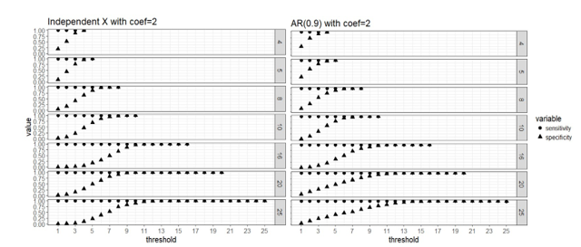
Figure 1. Strong signal scenario (regression coefficients are all equal to 2): sensitivity and specificity of the two-stage algorithm when training set are divided into  blocks respectively, and a variable is selected when  out of  blocks selects this predictor, where  =4, 5, 8, 10, 16, 20 and 25, = . Both the case with complete independence among predictors (left panel) and correlated predictors (right panel) are presented.

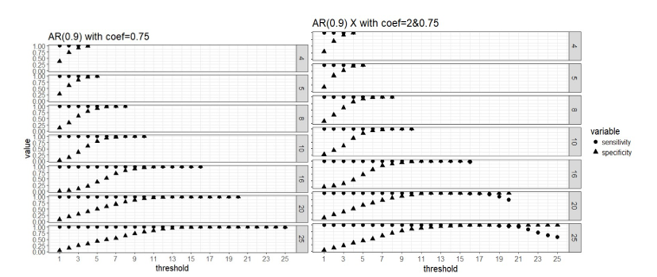
Figure 2. Weak signal scenario (regression coefficients are all equal to 0.75, left panel) and mixed signal scenario (regression coefficients are 0.75 or 2, right panel) with correlated predictors: sensitivity and specificity of the two-stage algorithm when training set are divided into  blocks respectively, and a variable is selected when  out of  blocks selects this predictor, where  =4, 5, 8, 10, 16, 20 and 25, = .

Apparently that when parallel computing is possible, it is computationally cheaper to divide the data into more blocks as there are less observations in each block and the computation speed is restricted by the computing cost of fitting the model to each block. Our simulation study did not use a real “BIG” sample size, so the computing time for each block is not high even when we use as low as 4 block. But in practice it is possible that we have giant training data and need to lower the computing cost of fitting a linear regression to a single block because the blocks still have large samples. All the number of blocks we considered here seem to approach the same level of sensitivity and specificity in variable selection, and it seems that 50% or higher blocks agreeing on the selection of variables is a good threshold for “majority voting.”

Four approaches are compared for the case of using 25 blocks on the data with independent predictors when the effect sizes are 2 (strong signal scenario).  

1. OLS: fit OLS with all 500 predictors to the original  
2. Split-resample: fit OLS with selected variables in the proposed approach to the original data
3. True p: fit OLS with the 100 “true signals” to the original data 
4. Split-resample: predict with aggregated estimation function in Chen and Xie (2014)

Comparison of the prediction performance can be visualized in the following figures:

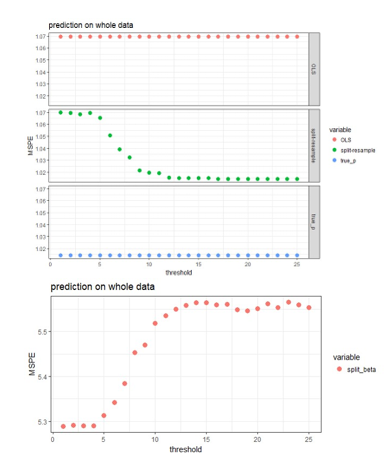
Figure 3: MSPE computed by refitting the model with selected variables to the original data and predict for the hold out test set.

The aggregated predictions result in much higher MSPE compared to the other three approaches, so it is shown in the lower panel of Figure 3, while the other three approaches are shown in the upper panel of Figure 3. The proposed approaches produces MSPE that approaches the best scenario when we know exactly which subset of the predictors are “true signals” in the simulated data when majority voting is used assuming 50% or higher proportion of blocks is the threshold of selecting predictors. It seems that the proposed algorithm works well in variable selection when the predictors are independent or correlated; and also predicts well when 50% or higher proportion of blocks is the threshold of selecting predictors. The smaller the effect size, the more blocks need to agree on variable selection in order to achieve the same sensitivity and specificity, but this 50% or higher threshold seem to work for both strong and weak signal case in general.

About the Author